
20 min read by Cloudmash
Evolution of AI So far...
It started by trying to mimic a neuron.
From One Neuron to Text-to-Video: The One Idea Behind All of AI
A child solves this puzzle in seconds. In 1969, it froze AI research for more than a decade.
Two switches. One bulb. The bulb turns on when exactly one switch is on. Not both. Not neither.
Your turn. Light the bulb.
The puzzle: light the bulb 1 of 4 states tried
Tap A and B. Find every way to turn it on.
| A | B | light |
|---|---|---|
| 0 | 0 | ? 0 |
| 0 | 1 | ? 1 |
| 1 | 0 | ? 1 |
| 1 | 1 | ? 0 |
Solved. Now the twist: a single artificial neuron can never learn this, no matter how long it trains. Machines only cracked it in 1986.
That fix started a chain of ideas that ends with models turning one sentence into a minute of video. See why the neuron fails.
Today, a model can turn one sentence into a minute of video. This post walks the whole road between that puzzle and that video, one step at a time.
And under every step sits the same idea. I will not tell you what it is yet. By the end, you will see it yourself.
Now look at how long each big leap in AI took.
Time between the big leaps
- Perceptron (1958) to learning XOR (1986) 28 years
- LSTM (1997) to Transformer (2017) 20 years
- Transformer (2017) to ChatGPT (2022) about 5 years
- ChatGPT (Nov 2022) to Sora (Feb 2024) about 15 months
From the first perceptron to networks that could learn XOR: 28 years. From the LSTM to the Transformer: 20 years. From the Transformer to ChatGPT: about 5 years. From ChatGPT to a model that turns one sentence into a minute of video: about 15 months.
The gaps keep shrinking. There is a reason for that, and it is the same idea I just promised you.
In this post 20 sections
- 1958: The Perceptron, a Machine That Draws One Line
- 1969: The XOR Problem That Froze Neural Networks
- 1986: Hidden Layers and Backpropagation
- 1990: Recurrent Neural Networks Give AI a Memory
- 1991: The Vanishing Gradient Problem
- 1997: LSTM, a Conveyor Belt Through Time
- LSTMs Already Did Translation, Captions and Speech
- Why LSTMs Hit a Wall, and Where Attention Came From
- 2017: Attention Is All You Need (the Transformer)
- Scale: BERT, GPT-3 and ChatGPT
- Encoders, Decoders and Embeddings
- The Central Insight: Encode Anything, Decode Anything
- Image to Text: Patches, Vision Transformers and CLIP
- Text to Image: How Diffusion Models Work
- Text to Video: Spacetime Patches, Sora and Veo 3
- The One Idea Behind All of AI
- What Comes Next: An Evolution We Cannot Imagine Yet
- Honest Caveats
- Frequently Asked Questions
- References and Further Reading
Today we walk that whole road. Start with one artificial neuron.
1958: The Perceptron, a Machine That Draws One Line
A perceptron is the simplest artificial neuron. It multiplies each input by a weight, adds the results together with a bias, and outputs 1 if the sum is above zero, otherwise 0. It learns by nudging its weights whenever it gets an answer wrong.
It started as an attempt to copy the brain. A real neuron collects signals from other cells, and if they add up to enough, it fires. Rosenblatt's 1958 paper is literally titled as a model of the brain.
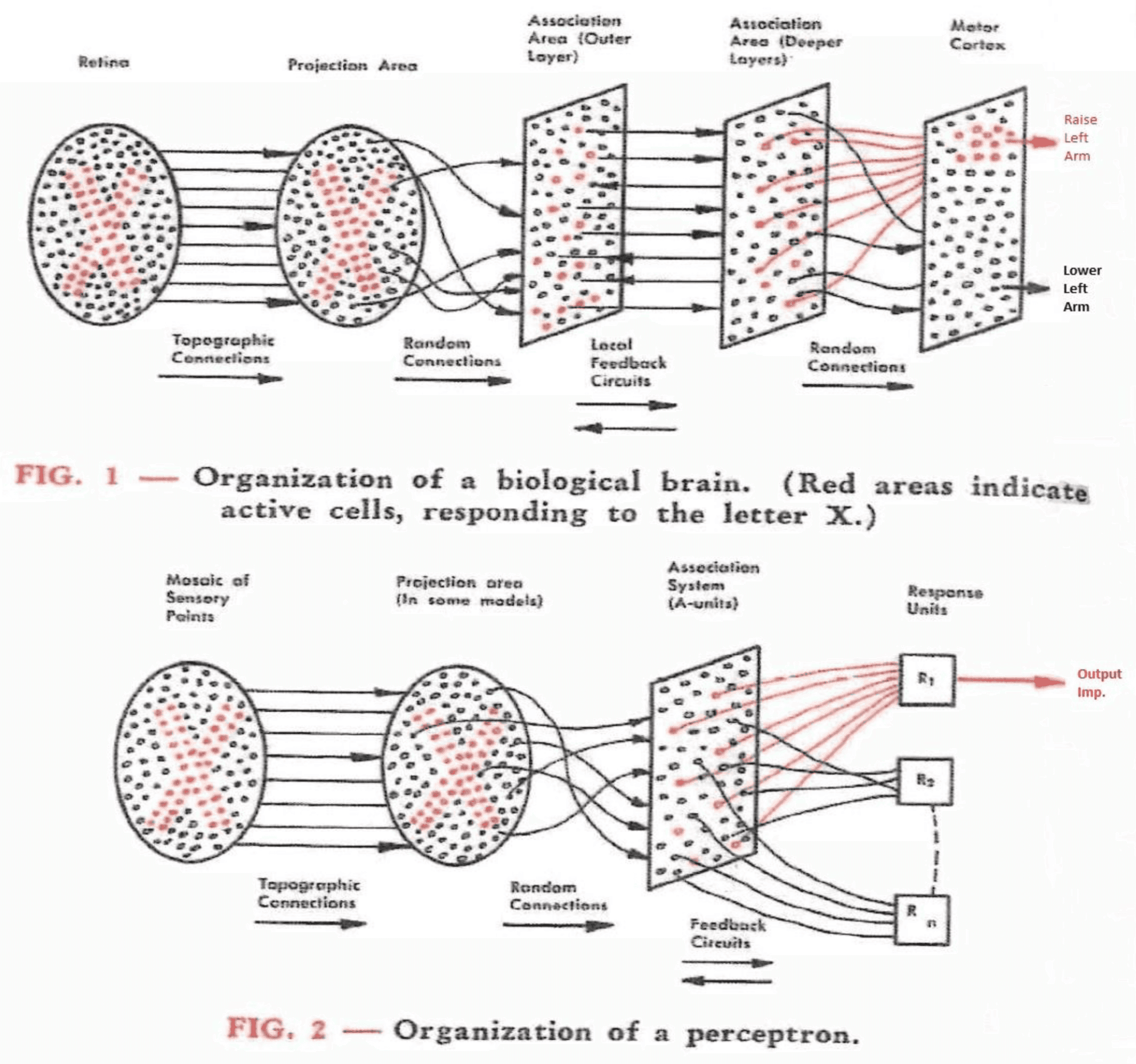

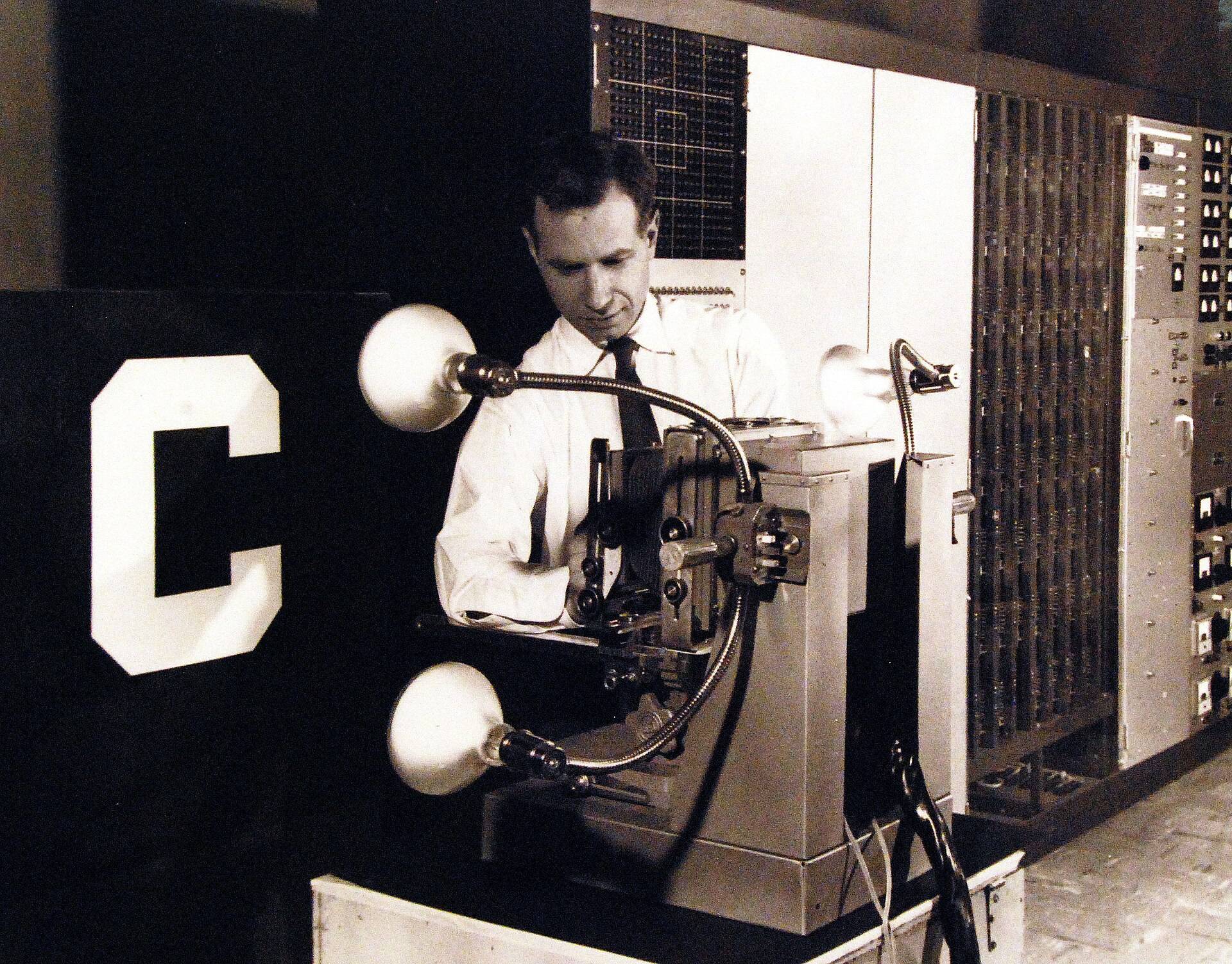
Frank Rosenblatt introduced the perceptron in 1958. Hardware followed: the Mark I Perceptron at Cornell Aeronautical Laboratory, with a 20 by 20 grid of light sensors. 400 photocells, looking at shapes.
_(20897323365).jpg)
Inputs times weights, plus a bias, then a step. That is the whole machine.
- teal: data moving forward
- orange: error moving backward
- violet: embedding space
- green: output 1
- red: output 0
It learns by correction. When an answer is wrong, nudge each weight toward the right answer. Repeat. That rule fits in three lines of Python:
X = np.array([[0, 0], [0, 1], [1, 0], [1, 1]])
GATES = {
    "AND": np.array([0, 0, 0, 1]),
    "OR":  np.array([0, 1, 1, 1]),
    "XOR": np.array([0, 1, 1, 0]),
}

def train_perceptron(X, y, epochs=50, lr=0.1):
    w, b = np.zeros(2), 0.0
    for _ in range(epochs):
        for xi, target in zip(X, y):
            pred = int(w @ xi + b > 0)          # weighted sum + bias, then a hard threshold
            error = target - pred               # -1, 0 or +1
            w += lr * error * xi                # nudge weights toward the right answer
            b += lr * error
    return w, b
show full file
"""A single perceptron learns AND and OR, but can never learn XOR.

Rosenblatt's rule: if the answer is wrong, nudge each weight toward the right answer.
Run: python 01_perceptron_xor_fails.py
"""
import numpy as np

X = np.array([[0, 0], [0, 1], [1, 0], [1, 1]])
GATES = {
    "AND": np.array([0, 0, 0, 1]),
    "OR":  np.array([0, 1, 1, 1]),
    "XOR": np.array([0, 1, 1, 0]),
}

def train_perceptron(X, y, epochs=50, lr=0.1):
    w, b = np.zeros(2), 0.0
    for _ in range(epochs):
        for xi, target in zip(X, y):
            pred = int(w @ xi + b > 0)          # weighted sum + bias, then a hard threshold
            error = target - pred               # -1, 0 or +1
            w += lr * error * xi                # nudge weights toward the right answer
            b += lr * error
    return w, b

for name, y in GATES.items():
    w, b = train_perceptron(X, y)
    preds = (X @ w + b > 0).astype(int)
    acc = (preds == y).mean()
    print(f"{name:3s}  predictions={preds}  target={y}  accuracy={acc:.0%}")
show output
AND  predictions=[0 0 0 1]  target=[0 0 0 1]  accuracy=100%
OR   predictions=[0 1 1 1]  target=[0 1 1 1]  accuracy=100%
XOR  predictions=[1 1 0 0]  target=[0 1 1 0]  accuracy=50%
Now the key picture. The weights and the bias define a straight line. Points on one side get a 1. Points on the other side get a 0.
w1 = 1, w2 = 1, b = -1.5
Only (1,1) lands on the green side. One line, all four right.
- output 1
- output 0
- the line
For AND, one line separates the answers. For OR, one line does it too. Same neuron, different weights. The line moves, but it is always a line.
So what happens when the answers cannot be split by one line?
1969: The XOR Problem That Froze Neural Networks
The XOR problem is the simplest task a single perceptron cannot learn. XOR outputs 1 when exactly one of two inputs is 1. On a grid, the two 1s sit on opposite corners and the two 0s on the other corners, and no single straight line can separate them.
Your turn. Drag the line and try to put both green dots on the shaded side and both red dots off it.
Try it: separate the 1s from the 0s with one line
Try any line you like. It always gets at least one point wrong.
A single perceptron can only draw one straight line. So it can never learn XOR. The code above agrees: trained on XOR, the same perceptron that aced AND and OR gets stuck at 50%.
This is not a training problem. More epochs will not fix it. The shape of the answer does not fit the shape of the model.
Perceptrons, by Marvin Minsky and Seymour Papert, 1969. Frost slides over the XOR grid.
In 1969, Marvin Minsky and Seymour Papert published a book called Perceptrons. It laid out limits like this one, and XOR became the famous example. Interest and funding for neural networks dried up. The field stayed cold for more than a decade.
The fix sounds simple. Use more than one neuron. Training them was the hard part.
1986: Hidden Layers and Backpropagation
Backpropagation is how a neural network with hidden layers learns. After each wrong answer, it uses the chain rule from calculus to send the error backward from the output, layer by layer, so that every weight learns how much it contributed to the mistake and which way to move.
The fix was to stack neurons. Add a hidden layer between the inputs and the output.
One hidden neuron draws one line. A second hidden neuron draws another. The output neuron combines them. Two lines carve out a band, and inside the band, XOR is 1.
You can try the same thing in the playground above: press "Give it a hidden layer" and the counter drops to zero.
That network is easy to draw. Training it was the hard part. When the output is wrong, which hidden weight is to blame? And by how much?
In 1986, Rumelhart, Hinton and Williams popularized the answer in Nature: backpropagation. It sends the error backward through the network, layer by layer, using the chain rule. Now every weight knows which way to move.
This is the fully connected network. Every neuron in one layer connects to every neuron in the next. With backprop, it learns XOR in a few lines of NumPy:
import numpy as np

rng = np.random.default_rng(1)
X = np.array([[0, 0], [0, 1], [1, 0], [1, 1]], dtype=float)
y = np.array([[0], [1], [1], [0]], dtype=float)

sigmoid = lambda z: 1 / (1 + np.exp(-z))

W1, b1 = rng.normal(size=(2, 2)), np.zeros((1, 2))   # input  -> 2 hidden neurons
W2, b2 = rng.normal(size=(2, 1)), np.zeros((1, 1))   # hidden -> 1 output neuron
lr = 1.0

for step in range(10_000):
    # forward pass
    h = sigmoid(X @ W1 + b1)
    out = sigmoid(h @ W2 + b2)

    # backward pass: the chain rule sends the error back, layer by layer
    d_out = (out - y) * out * (1 - out)
    d_h = (d_out @ W2.T) * h * (1 - h)

    W2 -= lr * h.T @ d_out;  b2 -= lr * d_out.sum(0, keepdims=True)
    W1 -= lr * X.T @ d_h;    b1 -= lr * d_h.sum(0, keepdims=True)

print("predictions:", out.round(3).ravel())   # close to [0, 1, 1, 0]
print("rounded:    ", out.round().astype(int).ravel())
show output
predictions: [0.013 0.989 0.989 0.011]
rounded:     [0 1 1 0]

But a network like this has no memory. And language is all memory.
1990: Recurrent Neural Networks Give AI a Memory
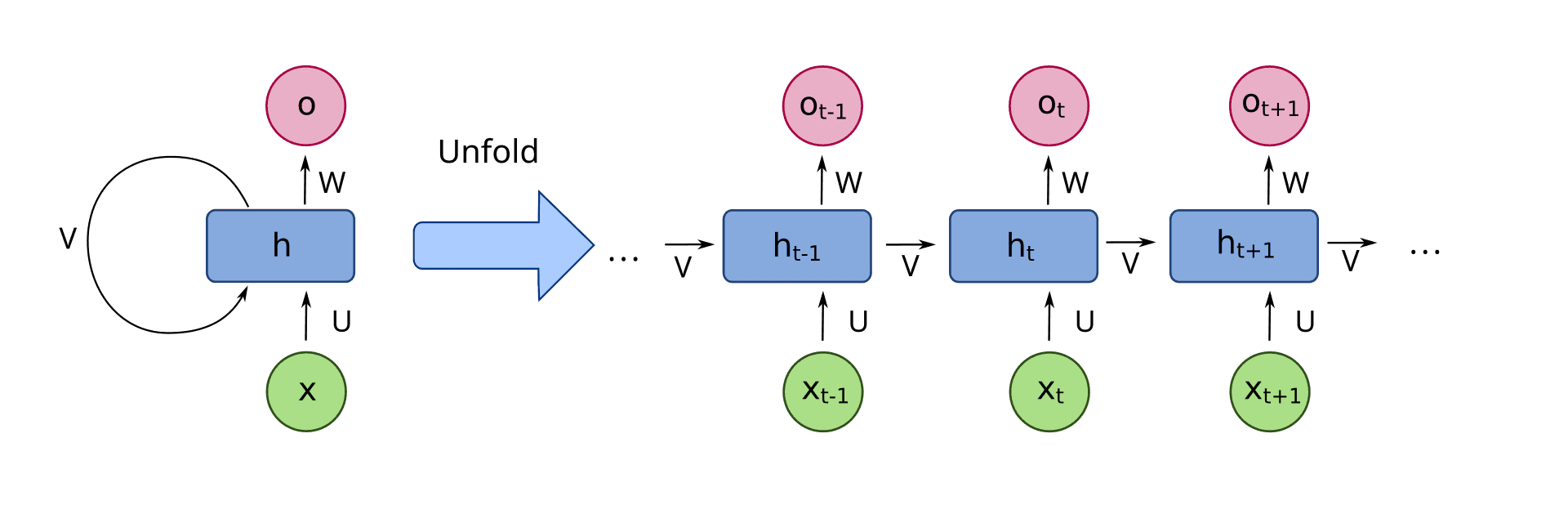
A recurrent neural network (RNN) reads a sequence one item at a time and keeps a hidden state: a small vector that summarizes everything it has read so far. At each step, it mixes the new input with the old state to make a new state, so earlier words can shape how later words are read.
A fully connected network takes a fixed-size input, all at once. Language does not work like that. The meaning of a word depends on the words before it.
Take "the cat that ate the fish was full". Who was full? To know, you have to remember "cat" across five other words.
The recurrent neural network fixes this. Watch it read, one word at a time:
folded: one cell, used again and again
hidden state h, first 4 of 16 numbers
unrolled: the same cell, once per word
- h1 the
- h2 cat
- h3 that
- h4 ate
- h5 the
- h6 fish
- h7 was
- h8 full
Jeffrey Elman's simple recurrent network, in "Finding Structure in Time" (1990), made this idea popular. The heart of it is one line of code:
import numpy as np

rng = np.random.default_rng(0)
vocab = "the cat that ate the fish was full".split()
emb = {w: rng.normal(size=8) for w in set(vocab)}    # a toy 8-dim vector per word

W_x = rng.normal(scale=0.3, size=(16, 8))   # how the new word enters
W_h = rng.normal(scale=0.3, size=(16, 16))  # how the old memory carries over
h = np.zeros(16)                            # the hidden state: memory of everything so far

for word in vocab:
    h = np.tanh(W_x @ emb[word] + W_h @ h)  # mix new word + old state -> new state
    print(f"{word:>5s}  h[:4] = {np.round(h[:4], 2)}")
show output
  the  h[:4] = [0.26 0.43 0.68 0.6 ]
  cat  h[:4] = [ 0.54  0.87  0.97 -0.72]
 that  h[:4] = [-0.04 -0.97  0.12  0.77]
  ate  h[:4] = [0.44 0.83 0.97 0.76]
  the  h[:4] = [ 0.35 -0.51  0.95 -0.45]
 fish  h[:4] = [-0.81 -0.57 -0.4   0.11]
  was  h[:4] = [-0.4  -0.18  1.   -0.73]
 full  h[:4] = [-0.48 -0.88 -0.94 -0.15]
Those are the same numbers the animation above shows in its hidden-state strip.

There is a catch hiding in that loop.
1991: The Vanishing Gradient Problem
The vanishing gradient problem is why plain recurrent networks forget. During training, the error signal is sent backward through every time step and shrinks a little at each one. After enough steps almost nothing is left, so the earliest words in a sequence receive almost no learning signal.
Training an RNN means sending the error backward through every time step. At each step, the gradient is multiplied by roughly the same factor. If that factor is below one, the signal shrinks.
Slide it out to 50 steps and watch.
0.9^10 = 0.3487
About 35% of the learning signal is left.
Point nine, multiplied by itself fifty times, is 0.0052. About half a percent. So the early words get almost no learning signal.
factor = 0.9
for steps in (1, 5, 10, 20, 30, 50):
    print(f"after {steps:2d} steps back: {factor ** steps:.4f}")
show output
after  1 steps back: 0.9000
after  5 steps back: 0.5905
after 10 steps back: 0.3487
after 20 steps back: 0.1216
after 30 steps back: 0.0424
after 50 steps back: 0.0052
Sepp Hochreiter analyzed this in 1991, in his diploma thesis at TU Munich, written in German. In practice, a plain RNN forgets anything more than a few words back.
The fix was not a better learning rule. It was a different shape of memory.
1997: LSTM, a Conveyor Belt Through Time
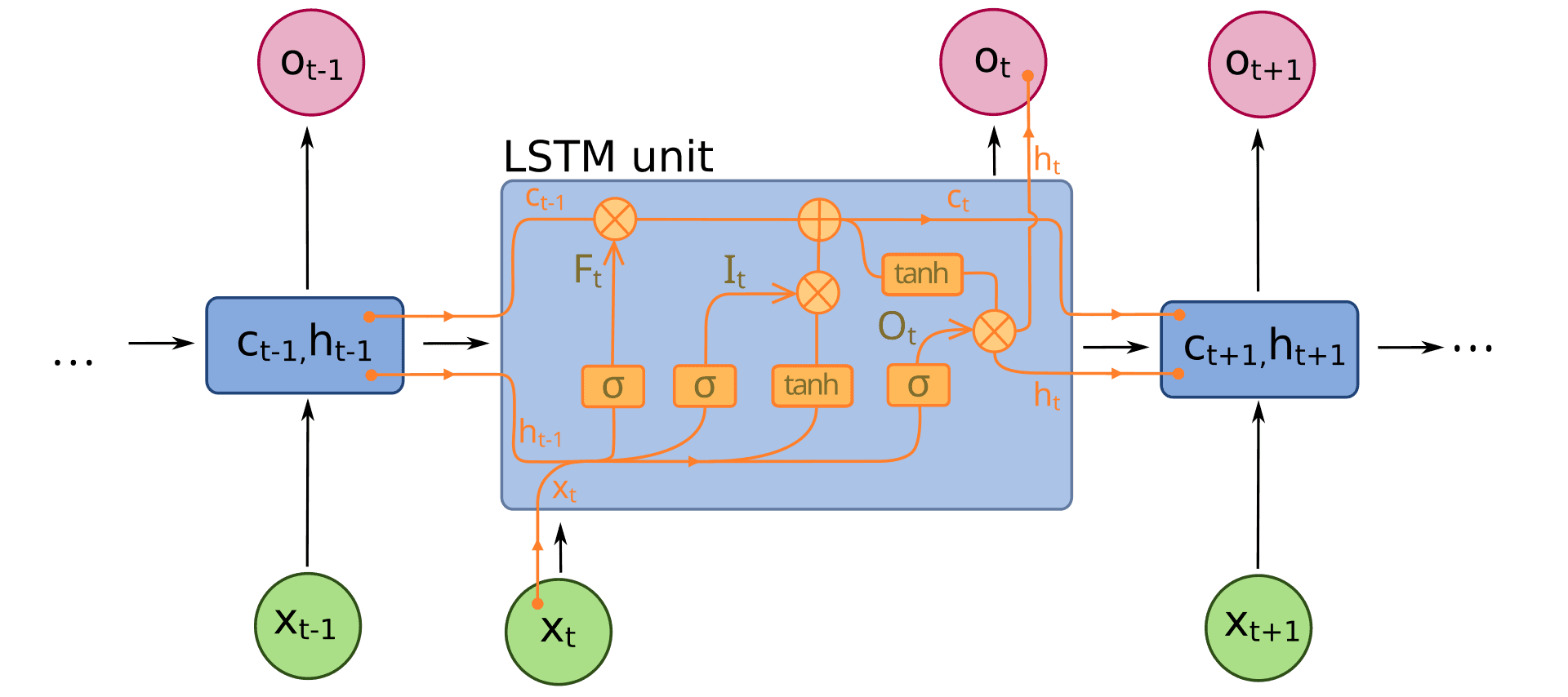
An LSTM (Long Short-Term Memory) is a recurrent network with a separate memory lane called the cell state. The cell state changes by addition instead of repeated multiplication, so the learning signal survives long sequences. Three gates decide what to erase from it, what to write to it, and what to reveal.
In 1997, Sepp Hochreiter and Juergen Schmidhuber introduced Long Short-Term Memory. The LSTM.
Think of the cell state as a conveyor belt running through time. Gates control the belt.
With the forget gate at 0.99, about 61% of the gradient survives 50 steps along the belt. A plain RNN keeps 0.5%.
- The forget gate decides what to erase.
- The input gate decides what to write.
- The output gate decides what to reveal.
Each gate is a small neuron that outputs a number between zero and one. Like a valve. The forget gate itself came a little later: Gers, Schmidhuber and Cummins added it in 2000.
def lstm_step(x, h, c, W, b):
    z = W @ np.concatenate([x, h]) + b
    f, i, o, g = np.split(z, 4)
    f, i, o = sigmoid(f), sigmoid(i), sigmoid(o)   # each gate outputs 0..1, like a valve
    g = np.tanh(g)                                 # candidate content to write

    c = f * c + i * g        # forget some old memory, ADD some new memory (no repeated multiply)
    h = o * np.tanh(c)       # reveal part of the memory as this step's output
    return h, c
show full file
import numpy as np

sigmoid = lambda z: 1 / (1 + np.exp(-z))

def lstm_step(x, h, c, W, b):
    z = W @ np.concatenate([x, h]) + b
    f, i, o, g = np.split(z, 4)
    f, i, o = sigmoid(f), sigmoid(i), sigmoid(o)   # each gate outputs 0..1, like a valve
    g = np.tanh(g)                                 # candidate content to write

    c = f * c + i * g        # forget some old memory, ADD some new memory (no repeated multiply)
    h = o * np.tanh(c)       # reveal part of the memory as this step's output
    return h, c

rng = np.random.default_rng(0)
d_in, d_hid = 8, 16
W = rng.normal(scale=0.2, size=(4 * d_hid, d_in + d_hid))
b = np.zeros(4 * d_hid)
h, c = np.zeros(d_hid), np.zeros(d_hid)
for t in range(5):
    h, c = lstm_step(rng.normal(size=d_in), h, c, W, b)
print("h:", h[:4].round(3), " c:", c[:4].round(3))
show output
h: [ 0.035 -0.031 -0.027 -0.095] c: [ 0.056 -0.063 -0.053 -0.177]Look at the line c = f * c + i * g. That plus sign is the whole trick.

The paper had a rocky start. At least, that is how Schmidhuber tells it:
"25th anniversary of the LSTM at #NeurIPS2021. reVIeWeR 2 - who rejected it from NeurIPS1995 - was thankfully MIA. The subsequent journal publication in Neural Computation has become the most cited neural network paper of the 20th century."
@SchmidhuberAI on X, Dec 6, 2021Keep an eye on that hidden state vector. It comes back.
LSTMs worked. So why did the field throw them out?
LSTMs Already Did Translation, Captions and Speech
Before Transformers, LSTMs already powered machine translation, image captioning, speech recognition and text generation. Google Translate ran on LSTMs from 2016. The tasks we now credit to modern AI were already solvable. What held LSTMs back was speed and scale, not ability.
Here is the part people forget. LSTMs already did much of what we now credit to modern AI.
- LSTM
Translation 2014, 2016
Sutskever, Vinyals and Le used two LSTMs to translate English to French (Seq2Seq). In 2016, Google Translate switched to the LSTM-based Google Neural Machine Translation system.
- LSTM
Image captioning 2014
Google's Show and Tell model captioned photos, with an LSTM writing the words.
- LSTM
Speech recognition on phones
Speech recognition on phones ran on LSTMs: sound in, one slice at a time, words out.
- LSTM
Text generation 2015
Andrej Karpathy showed an LSTM writing fake Shakespeare, one character at a time.
Karpathy's 2015 post is still worth reading. This is the kind of thing his LSTM wrote, one character at a time, after reading Shakespeare:
Fake Shakespeare, written by an LSTM one character at a time. It never saw a word, only letters.
Andrej Karpathy, The Unreasonable Effectiveness of Recurrent Neural Networks, May 2015That post has a fun footnote. Karpathy believes it is where the word "hallucination" for model mistakes got started:
"I believe this is true, I used the word in my 'Unreasonable Effectiveness of RNNs' post from 2015, and as far as I can remember I also hallucinated it."
@karpathy on X, Jul 27, 2025So what was the problem?
Why LSTMs Hit a Wall, and Where Attention Came From
Attention is a way for a model to look back at every part of its input and decide, for each output it produces, how much weight to give each part. It was first added to recurrent translation models in 2014, so they no longer had to squeeze a whole sentence into one vector.
Two problems.
First, an LSTM reads one step at a time. Step 50 must wait for step 49. You cannot spread that work across thousands of GPU cores.
LSTM: one step at a time
64 GPU cores
Second, everything squeezes through one hidden state. In translation, the whole source sentence was compressed into a single vector before the decoder wrote a word. Long sentences came out blurry.
The bottleneck: one vector for the whole sentence
The fix, 2014: attention
The first fix was attention. In 2014, Bahdanau, Cho and Bengio let the decoder look back at every encoder state and pick what to focus on, fresh for every word it writes.
Dzmitry Bahdanau was an intern at the time. Years later, he told the story in an email that Karpathy published. One line explains the whole motivation: "I was super skeptical about the idea of cramming a sequence of words in a vector."
"The (true) story of development and inspiration behind the "attention" operator, the one in "Attention is All you Need" that introduced the Transformer." Tap the image to read Bahdanau's full email.
@karpathy on X, Dec 3, 2024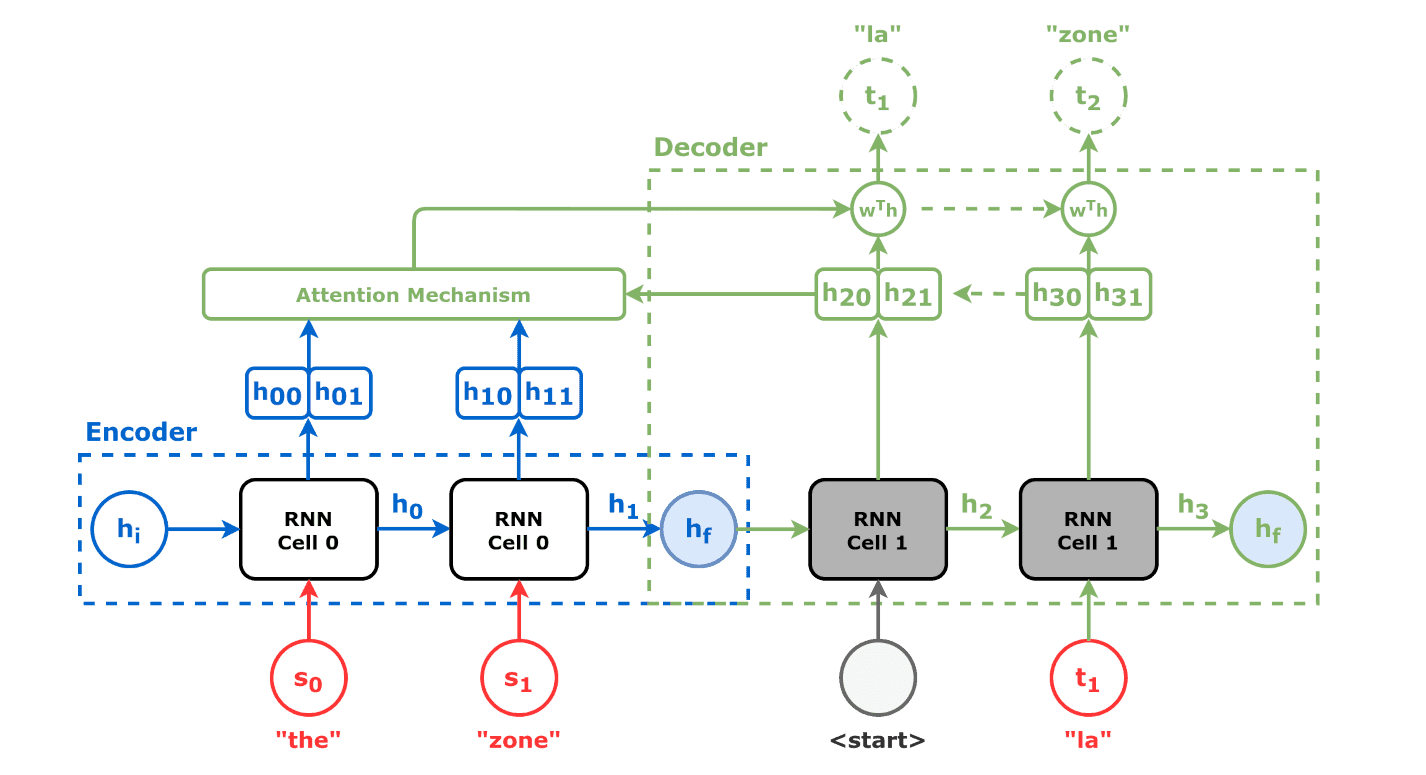

Then someone asked: what if attention is all you need?
2017: Attention Is All You Need (the Transformer)
A Transformer is a neural network that processes every word of its input at the same time. Each word uses attention to look at every other word and decide what to take from it. There is no recurrence, so training becomes large matrix multiplications, which GPUs run extremely fast.
In 2017, a team at Google published a paper with a bold title. Attention Is All You Need. The Transformer removed recurrence entirely.
Every word looks at every other word at the same time. To do that, each word makes three vectors:
- a query: what am I looking for?
- a key: what do I contain?
- a value: what will I pass on?
The match between one word's query and another word's key decides how much of that word's value flows in. Try it. Switch the last word from "tired" to "wide" and watch where "it" looks.
The animal didn't cross the street because it was too tired.
- The
- animal
- didn't
- cross
- the
- street
- because
- it
- was
- tired
Here is the real thing, from Google's 2017 announcement. With "tired", "it" attends to "animal". With "wide", it attends to "street".
The same sentence, two endings, two different targets for "it". Nobody wrote that rule. The model learned it.
Google Research blog, 2017All of it is matrix multiplication. Three multiplies to make Q, K and V. One to compare every query with every key. One more to blend the values.
def self_attention(X, Wq, Wk, Wv):
    Q, K, V = X @ Wq, X @ Wk, X @ Wv          # three matrix multiplies
    scores = Q @ K.T / np.sqrt(K.shape[-1])   # every query against every key
    weights = softmax(scores)                 # each row sums to 1
    return weights @ V, weights               # blend the values
show full file
import numpy as np

def softmax(z):
    z = z - z.max(-1, keepdims=True)
    e = np.exp(z)
    return e / e.sum(-1, keepdims=True)

def self_attention(X, Wq, Wk, Wv):
    Q, K, V = X @ Wq, X @ Wk, X @ Wv          # three matrix multiplies
    scores = Q @ K.T / np.sqrt(K.shape[-1])   # every query against every key
    weights = softmax(scores)                 # each row sums to 1
    return weights @ V, weights               # blend the values

rng = np.random.default_rng(0)
tokens = "The animal didn't cross the street because it was tired".split()
d = 16
X = rng.normal(size=(len(tokens), d))
Wq, Wk, Wv = (rng.normal(scale=d ** -0.5, size=(d, d)) for _ in range(3))

out, w = self_attention(X, Wq, Wk, Wv)
print("output shape:", out.shape)             # (10, 16): one new vector per word, computed in parallel
print("weights from 'it':", {t: float(v) for t, v in zip(tokens, w[tokens.index("it")].round(2))})
# With random weights the pattern is random. A trained model learns to put the
# biggest weight from "it" on "animal".
show output
output shape: (10, 16)
weights from 'it': {'The': 0.25, 'animal': 0.13, "didn't": 0.01, 'cross': 0.02, 'the': 0.16, 'street': 0.01, 'because': 0.25, 'it': 0.08, 'was': 0.01, 'tired': 0.08}
No word waits for another. Every row is computed at once.
Transformer: every word at once
64 GPU cores
GPUs are built for exactly that. So training could finally scale to a large part of the internet.
Five years later, Karpathy summed up why the design won:
"The Transformer is a magnificient neural network architecture because it is a general-purpose differentiable computer. It is simultaneously: 1) expressive (in the forward pass) 2) optimizable (via backpropagation+gradient descent) 3) efficient (high parallelism compute graph)"
@karpathy on X, Oct 19, 2022Notice what every step so far has in common. We are close.
Then scale took over.
Scale: BERT, GPT-3 and ChatGPT
After the Transformer, progress came mostly from scale: the same basic block, stacked deeper and trained on more data. Parameter counts went from 117 million in GPT-1 (2018) to 175 billion in GPT-3 (2020). ChatGPT, launched on November 30, 2022, put that scale in front of everyone.
Parameters, log scale
- GPT-1 2018 117M
- BERT-Large 2018 340M
- GPT-2 2019 1.5B
- GPT-3 2020 175B
Then ChatGPT, November 30, 2022
Language models were not new. They just had not mattered much yet. Karpathy, less than two weeks before ChatGPT:
"An interesting historical note is that neural language models have actually been around for a very long time but noone really cared anywhere near today's extent."
@karpathy on X, Nov 18, 2022Then this happened:
"Try talking with ChatGPT, our new AI system which is optimized for dialogue."
@OpenAI on X, Nov 30, 2022"ChatGPT launched on wednesday. today it crossed 1 million users!"
@sama on X, Dec 5, 2022To see what came next, go back to translation.
Encoders, Decoders and Embeddings
Here it is. The idea this whole post has been circling.
An encoder-decoder has two halves. The encoder reads the input and turns it into a list of numbers. The decoder reads those numbers and produces the output.
That list of numbers is the embedding. Hover over the words on the map.
cat: nearest are dog and kitten. Far from car.
King sits near queen. Cat sits near dog. Far from car. Closeness is measured with plain geometry, usually the angle between two vectors:
import numpy as np

E = {            # [royalty, animal, vehicle]
    "king":  np.array([0.95, 0.05, 0.00]),
    "queen": np.array([0.93, 0.08, 0.02]),
    "cat":   np.array([0.02, 0.97, 0.03]),
    "dog":   np.array([0.03, 0.95, 0.06]),
    "car":   np.array([0.01, 0.04, 0.98]),
}

def cos(a, b):
    return a @ b / (np.linalg.norm(a) * np.linalg.norm(b))

for a, b in [("king", "queen"), ("cat", "dog"), ("cat", "car")]:
    print(f"cos({a}, {b}) = {cos(E[a], E[b]):.2f}")
show output
cos(king, queen) = 1.00
cos(cat, dog) = 1.00
cos(cat, car) = 0.07
Real models learn these numbers instead of being handed them, and use hundreds or thousands of dimensions instead of three. The idea is the same.
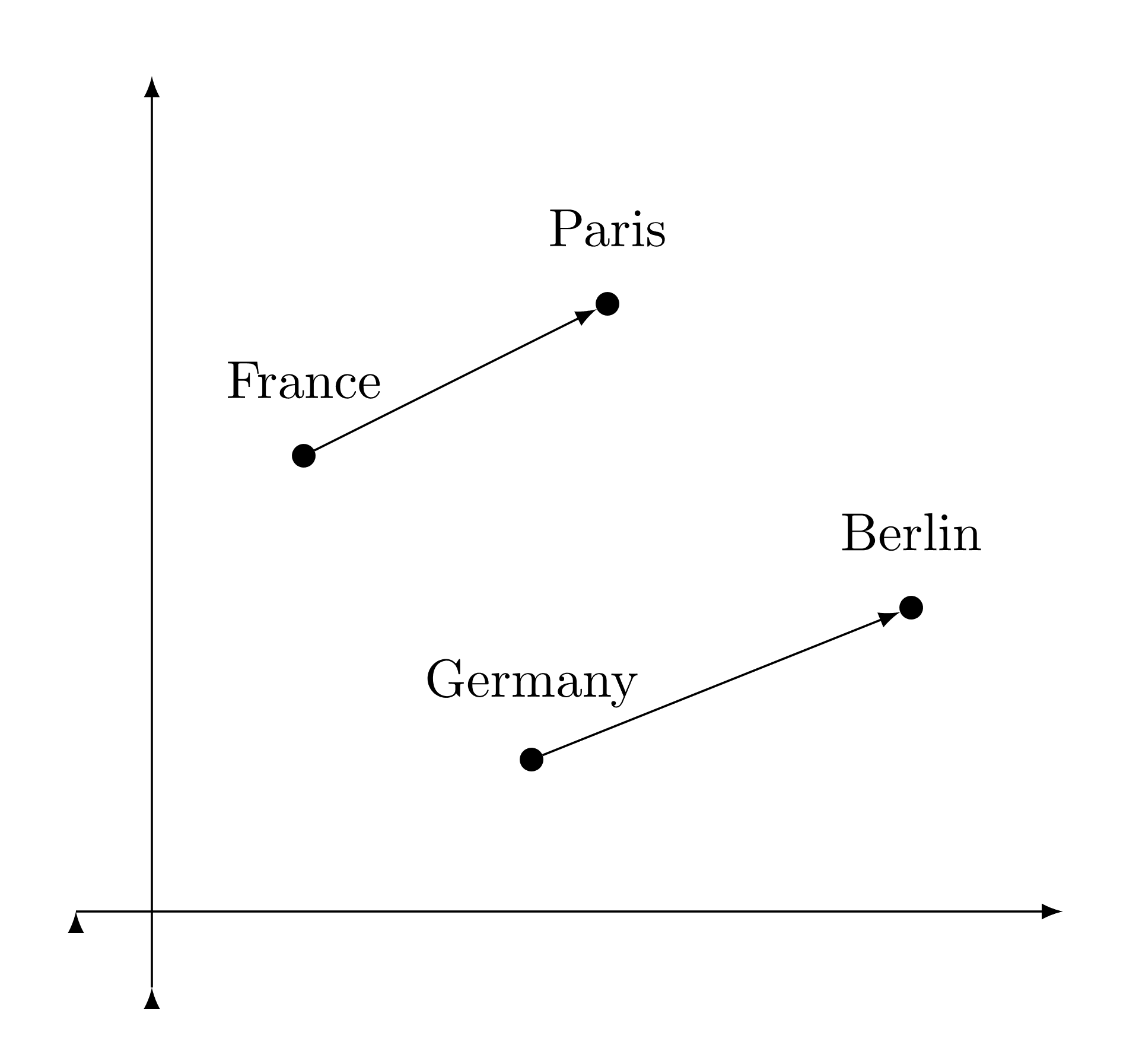

Now look at what that unlocks.
The Central Insight: Encode Anything, Decode Anything
Modern multimodal AI rests on one move: turn any kind of input into embedding vectors, then decode those vectors into any kind of output. If images, text, audio and video can all be encoded into the same kind of vector space, a model can translate between them the way it translates between languages.
Here is the central insight. The encoder does not have to read text. The decoder does not have to write text.
If you can encode an image into the same kind of vector, you can decode it into a sentence. If you can encode a sentence, you can decode it into pixels. Or into frames of video.
Image in, text out
The rest of the road is that one picture, three times.
Start with image to text.
Image to Text: Patches, Vision Transformers and CLIP
A Vision Transformer (ViT) reads an image the way a Transformer reads a sentence. It cuts the image into small square patches, turns each patch into a vector, and feeds the row of vectors to a Transformer. A text decoder can then attend to those patch vectors and write words about the image.
Image to text first. This is the Vision Transformer, from October 2020:
1 An image
text decoder
The decoder attends to the patch vectors exactly like a translation decoder attending to French. In code, "cut into patches" is a single reshape:
import numpy as np

# An image: 224 x 224 pixels, 3 color channels
img = np.zeros((224, 224, 3))
p = 16
patches = img.reshape(224 // p, p, 224 // p, p, 3).transpose(0, 2, 1, 3, 4).reshape(-1, p * p * 3)
print("image patches:", patches.shape)        # (196, 768): 196 tokens, one vector each
show output
image patches: (196, 768)In January 2021, OpenAI's CLIP learned from 400 million image and caption pairs. It pulled each image and its caption to the same spot in embedding space. A photo of a dog and the words "a photo of a dog" end up as neighbors.
OpenAI announced CLIP together with something that ran the arrow the other way:
"We've developed two neural networks which have learned by associating text and images. CLIP maps images into categories described in text, and DALL-E creates new images, like this, from text."
@OpenAI on X, Jan 5, 2021Today, GPT-4o, Gemini and Claude can read a photo, a chart or a handwritten note, and answer questions about it.
Now reverse the arrow.
Text to Image: How Diffusion Models Work
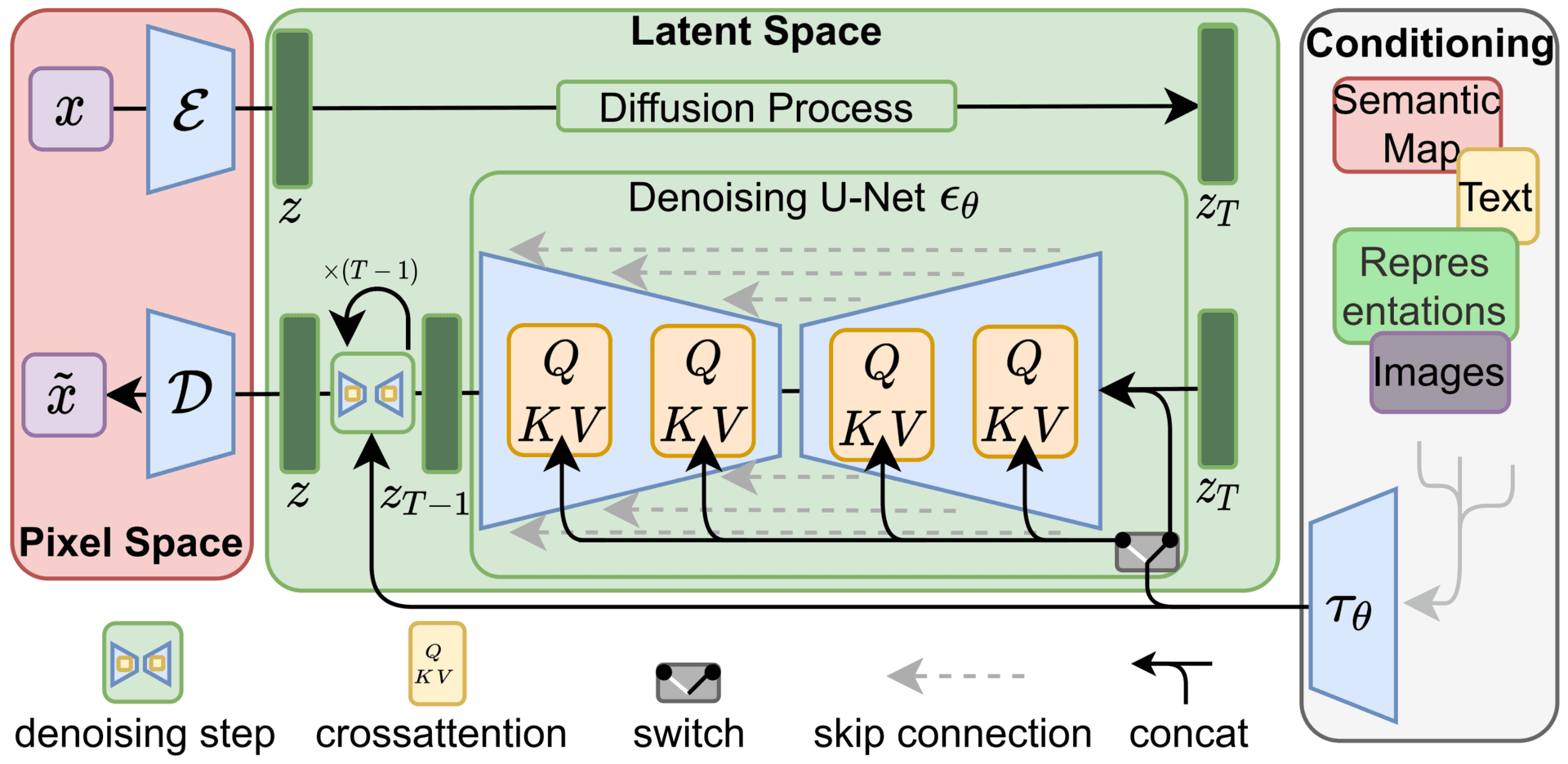
A diffusion model generates an image by removing noise. In training, real images get noise added step by step, and the model learns to undo one step. To generate, it starts from pure static and denoises again and again, while the text embedding steers what the picture becomes.
Text to image. In January 2021, OpenAI's DALL-E drew an armchair in the shape of an avocado.
The image everyone remembers. Nobody had photographed these chairs. They did not exist.
OpenAI, DALL-E: Creating images from text, 2021In 2022 came DALL-E 2, Midjourney and Stable Diffusion. Most of these use diffusion.


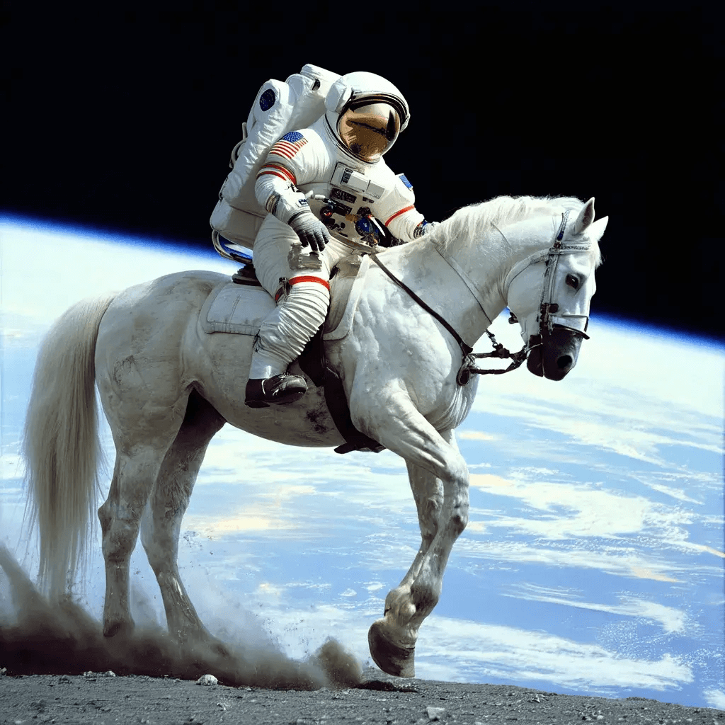
.webp)
Here is how diffusion works. In training, you take a real image and add noise, step by step, until only static is left. The model learns to undo one step of noise.
import numpy as np

T = 1000
betas = np.linspace(1e-4, 0.02, T)          # the DDPM noise schedule (Ho et al., 2020)
a_bar = np.cumprod(1 - betas)               # how much of the original image survives

def add_noise(x0, t, rng):
    noise = rng.normal(size=x0.shape)
    return np.sqrt(a_bar[t]) * x0 + np.sqrt(1 - a_bar[t]) * noise, noise

for t in (0, 100, 250, 500, 999):
    print(f"t={t:4d}  signal kept={np.sqrt(a_bar[t]):.3f}")
# t=999: almost pure static. The model is trained to predict `noise` from (x_t, t, text embedding).
show output
t=   0  signal kept=1.000
t= 100  signal kept=0.946
t= 250  signal kept=0.722
t= 500  signal kept=0.279
t= 999  signal kept=0.006
To generate, start from pure static. Remove noise again and again. At every step, the text embedding steers what the picture becomes. Scrub through it:
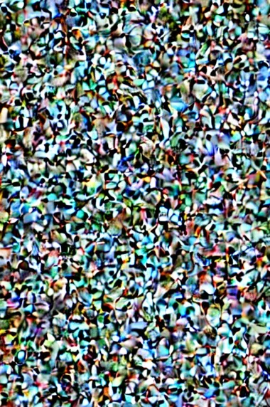

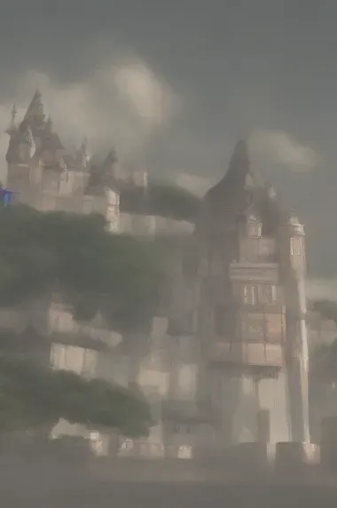



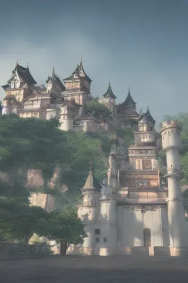
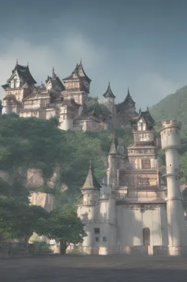 1 step
 prompta European-style castle in Japan
training add noise, step by step, until only static is left
generating remove noise, step by step, with the text embedding steering every step

Stable Diffusion does all this in a compressed latent space instead of on full-size pixels. So it runs on a home graphics card.

Text to video adds one more dimension. Time.
Text to Video: Spacetime Patches, Sora and Veo 3
Text-to-video models like Sora treat a video as a stack of frames and cut it into spacetime patches: small cubes of pixels that span several frames. A diffusion transformer starts from noise and denoises all of the patches together, which is how the frames stay consistent with each other.
A video is a stack of frames. And the frames must agree with each other. A ball cannot jump across the screen between two frames, and a cat cannot change color.
Meta showed Make-A-Video in September 2022. Runway released Gen-2 in 2023. Then, on February 15, 2024, OpenAI showed Sora.
"Introducing Sora, our text-to-video model. Sora can create videos of up to 60 seconds featuring highly detailed scenes, complex camera motion, and multiple characters with vibrant emotions."
@OpenAI on X, Feb 15, 2024Here is what one spacetime patch looks like:
OpenAI's technical report draws the same picture:
Frames go in, a visual encoder compresses them, and the result is cut into spacetime patches: the video version of image patches.
OpenAI, Video generation models as world simulators, 2024In code, it is the image reshape from before with one more axis. Time:
# A video: 16 frames of 224 x 224 x 3
video = np.zeros((16, 224, 224, 3))
t, p = 4, 16                                  # each cube spans 4 frames and 16x16 pixels
cubes = (video.reshape(16 // t, t, 224 // p, p, 224 // p, p, 3)
              .transpose(0, 2, 4, 1, 3, 5, 6)
              .reshape(-1, t * p * p * 3))
print("spacetime patches:", cubes.shape)      # (784, 3072): small cubes of pixels across time
show output
spacetime patches: (784, 3072)In May 2025, Google DeepMind's Veo 3 generated video and its sound together, in one model.
"Video, meet audio. With Veo 3, our new state-of-the-art generative video model, you can add soundtracks to clips you make."
@GoogleDeepMind on X, May 20, 2025So look back at the whole road.
The One Idea Behind All of AI
One neuron that could only draw one line. Layers that could draw many. Recurrence that gave memory. Gates that kept memory alive. Attention that let everything look at everything, in parallel.
And under all of it, one idea.
- Perceptron
- XOR wall
- Backprop
- RNN
- Vanishing gradient
- LSTM
- Seq2Seq + attention
- Transformer
- ChatGPT
- CLIP
- Stable Diffusion
- Sora
Turn the world into vectors.
Learn to move between them.
Encode anything. Decode into anything.
Image in, text out
The hidden state of an RNN was a vector. The LSTM's memory was a vector. Attention compared vectors. An embedding is a vector. A patch of an image, a cube of video, a word: all vectors, all in spaces a model can move through.
The gaps between breakthroughs went from decades to months. Because each step stood on the last.
So where does the road go from here?
What Comes Next: An Evolution We Cannot Imagine Yet
Nobody knows where AI goes next. But the one idea in this post gives a useful way to look: anything that can be turned into vectors can be connected to anything else. The open question is what else can be encoded, and what it can be decoded into.
It all started by trying to mimic a single neuron. One weighted sum. One straight line. Nobody building the Mark I in a lab at Cornell could have pictured a sentence turning into a minute of video.
Now point the same idea at new kinds of input and output:
- already here
a protein sequence its 3D shape
A protein is a sentence in a 20-letter alphabet. AlphaFold reads it and predicts the folded shape. Its creators shared the 2024 Nobel Prize in Chemistry.
- early research
camera + words robot movements
Encode what a robot sees and what you asked for. Decode into motor commands. Researchers already train models like this.
- early research
brain signals text
Early experiments decode recorded brain activity into words. The field began by copying a neuron. Now it is learning to read them.
- early research
a sentence a whole world
OpenAI called its video models "world simulators". Next: worlds you can walk through and change, not just watch.
- open question
all of science a new discovery
Encode every paper, measurement and failed experiment. Decode into a hypothesis nobody has tested. Can a model find what we missed?
- not imagined yet
? ?
In 1958, nobody working on the perceptron could picture a minute of video made from a sentence. The most important card on this list is the one nobody can write yet.
- already here
- early research
- open question
Some of these are already here. Some are early research. Some are only questions. And if this history teaches anything, the biggest change will be the one that is not on the list.
The gaps between breakthroughs went from 28 years to about 15 months. Nobody can say how short the next one will be.
Honest Caveats
A few honest caveats, because a clean story always leaves things out.
- 1
One path, not the whole map
Convolutional networks, reinforcement learning and many other ideas mattered just as much. This post follows one thread.
- 2
LSTMs are not dead
They still run in small, streaming and low-power settings, where reading one step at a time is a feature.
- 3
One shared space is a picture
A single shared embedding space is a useful picture. Real systems often glue separately trained parts together.
Frequently Asked Questions
What is the XOR problem in neural networks?
XOR outputs 1 when exactly one of two inputs is 1. Plot the four input pairs on a grid and the two 1s sit on opposite corners, with the two 0s on the other corners. No single straight line can separate them, so a single perceptron cannot learn XOR. Minsky and Papert laid out limits like this in 1969.
Why couldn't a single perceptron learn XOR?
A perceptron is a weighted sum plus a threshold, so it can only ever draw one straight line between its 1s and its 0s. XOR needs two lines: one to cut off (0,0) and one to cut off (1,1). A hidden layer gives two neurons, two lines, and a band between them that holds both 1s.
What is the vanishing gradient problem?
When a recurrent network learns, the error is sent backward through every time step and multiplied by roughly the same factor at each one. If that factor is below one, the signal shrinks fast: 0.9 multiplied by itself 50 times is about 0.005. The earliest words get almost no learning signal. Sepp Hochreiter analyzed this in 1991.
How is an LSTM different from an RNN?
A plain RNN rewrites one hidden state at every step. An LSTM adds a separate cell state that changes by addition instead of repeated multiplication, so the gradient can flow back along it without vanishing. Three gates, forget, input and output, each output a number between 0 and 1 and decide what to erase, write and reveal.
Why did Transformers replace LSTMs?
An LSTM reads one step at a time, so step 50 waits for step 49 and most GPU cores sit idle. It also squeezes everything through one hidden state. A Transformer lets every word attend to every other word at the same time, using matrix multiplication, which is exactly what GPUs are built for. So training could scale.
What is an embedding in AI?
An embedding is a list of numbers that places a word, image or sound as a point in a space with hundreds or thousands of dimensions. Similar meanings land close together: king near queen, cat near dog, far from car. Encoders turn inputs into embeddings, and decoders turn embeddings back into text, images or video.
How does text-to-image AI work?
Most text-to-image models use diffusion. In training, noise is added to real images step by step, and the model learns to undo one step of it. To generate, the model starts from pure static and removes noise again and again, with the text embedding steering every step. Stable Diffusion does this in a compressed latent space.
How does Sora generate video?
Sora cuts video into spacetime patches: small cubes of pixels that span several frames. A diffusion transformer starts from noise and denoises all the patches together, which keeps the frames consistent with each other. OpenAI showed Sora on February 15, 2024, generating clips of up to 60 seconds.
References and Further Reading
The perceptron era
- F. Rosenblatt, 1958. "The Perceptron: A Probabilistic Model for Information Storage and Organization in the Brain." Psychological Review. DOI
- M. Minsky, S. Papert, 1969. "Perceptrons." MIT Press.
Learning and memory
- D. Rumelhart, G. Hinton, R. Williams, 1986. "Learning representations by back-propagating errors." Nature. DOI
- J. Elman, 1990. "Finding Structure in Time." Cognitive Science. DOI
- S. Hochreiter, 1991. "Untersuchungen zu dynamischen neuronalen Netzen." Diploma thesis, TU Munich. PDF
- S. Hochreiter, J. Schmidhuber, 1997. "Long Short-Term Memory." Neural Computation 9(8). DOI
- F. Gers, J. Schmidhuber, F. Cummins, 2000. "Learning to Forget: Continual Prediction with LSTM." Neural Computation. DOI
- R. Pascanu, T. Mikolov, Y. Bengio, 2012. "On the difficulty of training Recurrent Neural Networks." arXiv 1211.5063
Sequences, attention and the Transformer
- I. Sutskever, O. Vinyals, Q. Le, 2014. "Sequence to Sequence Learning with Neural Networks." arXiv 1409.3215
- D. Bahdanau, K. Cho, Y. Bengio, 2014. "Neural Machine Translation by Jointly Learning to Align and Translate." arXiv 1409.0473
- O. Vinyals et al., 2014. "Show and Tell: A Neural Image Caption Generator." arXiv 1411.4555
- A. Karpathy, 2015. "The Unreasonable Effectiveness of Recurrent Neural Networks." Blog post
- Y. Wu et al., 2016. "Google's Neural Machine Translation System." arXiv 1609.08144
- A. Vaswani et al., 2017. "Attention Is All You Need." arXiv 1706.03762
Scale
- J. Devlin et al., 2018. "BERT: Pre-training of Deep Bidirectional Transformers for Language Understanding." arXiv 1810.04805
- T. Brown et al., 2020. "Language Models are Few-Shot Learners." arXiv 2005.14165
Images and video
- A. Dosovitskiy et al., 2020. "An Image is Worth 16x16 Words: Transformers for Image Recognition at Scale." arXiv 2010.11929
- A. Radford et al., 2021. "Learning Transferable Visual Models From Natural Language Supervision." arXiv 2103.00020
- A. Ramesh et al., 2021. "Zero-Shot Text-to-Image Generation." arXiv 2102.12092
- J. Ho, A. Jain, P. Abbeel, 2020. "Denoising Diffusion Probabilistic Models." arXiv 2006.11239
- R. Rombach et al., 2021. "High-Resolution Image Synthesis with Latent Diffusion Models." arXiv 2112.10752
- U. Singer et al., 2022. "Make-A-Video: Text-to-Video Generation without Text-Video Data." arXiv 2209.14792
- W. Peebles, S. Xie, 2022. "Scalable Diffusion Models with Transformers." arXiv 2212.09748
- OpenAI, 2024. "Video generation models as world simulators." Report
Further reading
- C. Olah, 2015. "Understanding LSTM Networks." colah.github.io
- J. Alammar, 2018. "The Illustrated Transformer." jalammar.github.io
The XOR puzzle was solved long ago. The bigger puzzles are still open.